How to create/use a spreadsheet in Google Drive with the current prices of your cryptocoins

Today I had to create a spreadsheet to manage my cryptocoins portfolio.

Later this month I will create a Dashboard Web to show this information more easily and beautifully, as well as providing various reports. But while it's not ready I've created a spreadsheet to advance the service and by doing so I've discovered a very useful Add-on for anyone who wants to manage their profits on top of those digital assets.

---

Add-on - CRYPTOFINANCE

This add-on is the simplest way to provide the current value of any cryptocoin on the market, only needing to use the function/formula:

=CRYPTOFINANCE("ADA/BTC")

Function - TEXTJOIN

While I was creating the lines of each coin, I asked myself:

Is there an automatic way to create the "COIN/BTC" String? I already have the symbol for each one in the first column.

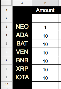
So I searched Google and found the following link:

• https://support.google.com/docs/table/25273?visit_id=1-636544947571461454-1779998409&hl=en&rd=2

And I just searched for: join. Because I knew it should be something like that.

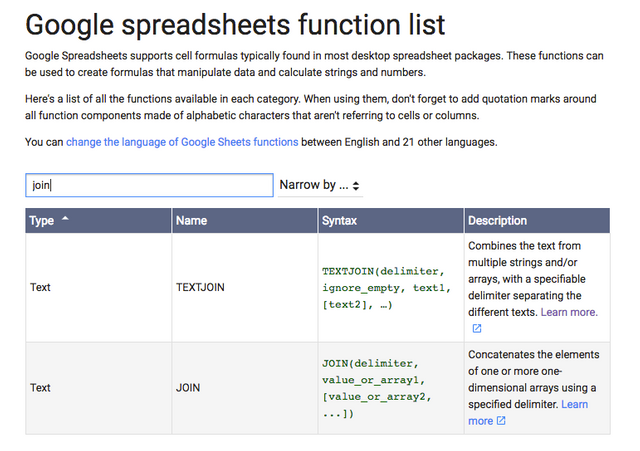
Then I just analyzed which function would be the best for my problem and chose TEXTJOIN because I do not need several values like JOIN that accepts an Array of values.

In this way I was able to create a function that searches the value of the currency that has its symbol in column A:

=CRYPTOFINANCE(TEXTJOIN("/", TRUE, A3, "BTC"))

For you to be able to reuse this same formula in the other rows of the worksheet just do the same action you would do in Excel, just click and hold in the lower right corner of the cell and drag stop down to the desired end line, because thus the value of A3 will only change the line number and not the column.

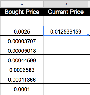
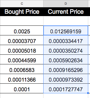
Now you can reuse it whenever you want!

---

Bonus

Function - Current Value

In this function we need to fix which is the cell that has the Bitcoin Current Price, which is H2, so that we can multiply by the Amount result times the Current Price.

• Amount: B{3};
• Current Price: D{3};
• Bitcoin Current Price: H2;

To fix the Bitcoin Current Price cell we will use $, thus leaving: $H$2.

In this way we have fixed that it will always be the H column and always the 2 cell:

=(B3*D3)*$H$2

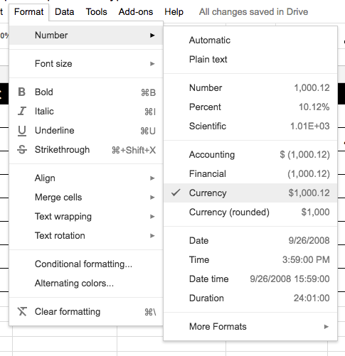
Tip - Format

Properly format your column if it is not as currency:

Function - Profit

Before showing this formula I will show how we can deduce it.

Imagine that the value bought was 200 and the current value is 220, or 10% of profit.

We take the difference between the initial value and the final value, note here that if the final value is greater than the initial value, then having profit, the result will be a negative value:

=(200-220) // = -20

With the difference we will know the proportion of this value to the initial value, making a simple division:

=(200-220)/200 // = -20 / 200 = -0.1

And since we know that Profit should be positive, we need to multiply by -1:

=(200-220)/200*-1 // = -20 / 200 = -0.1 * -1 = 0.1

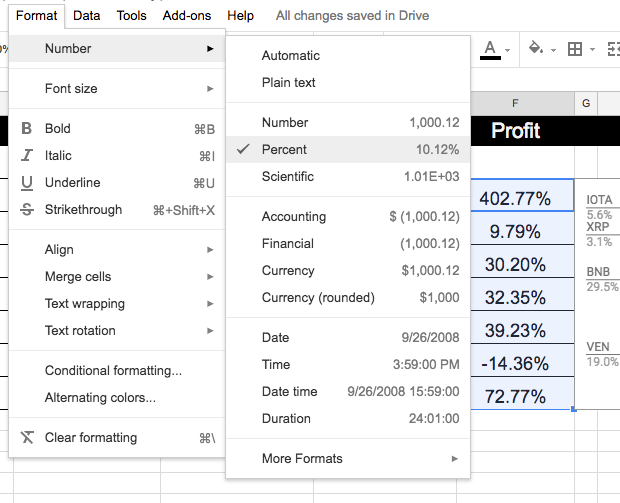
I just did not add one more multiplication per 100, so we have the actual percentage, because we will format this column in a similar way to what we did with Current Value, so we created the following formula:

=(initial-final)/initial*-1

Changing our cells was like this:

=(C9-D9)/C9*-1

Tip - Format

---

Example - How to use?

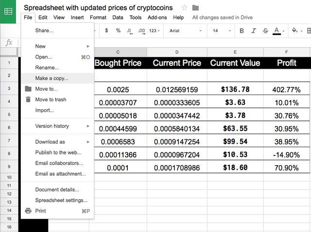
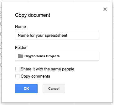
You can use my running example creating a copy of it.

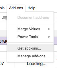
Add the Add-on to your spreadsheet:

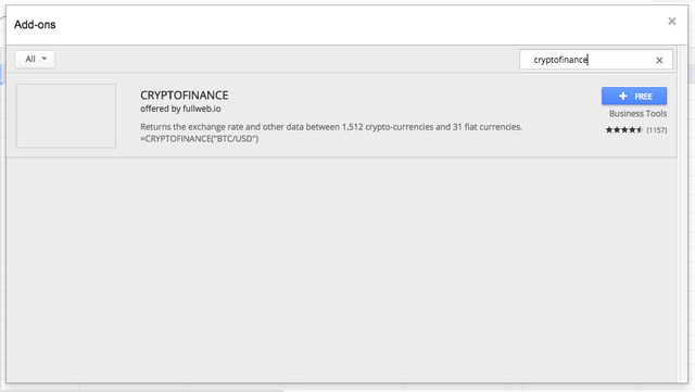
Search for the Add-on and add it:

Then just wait to load the data:

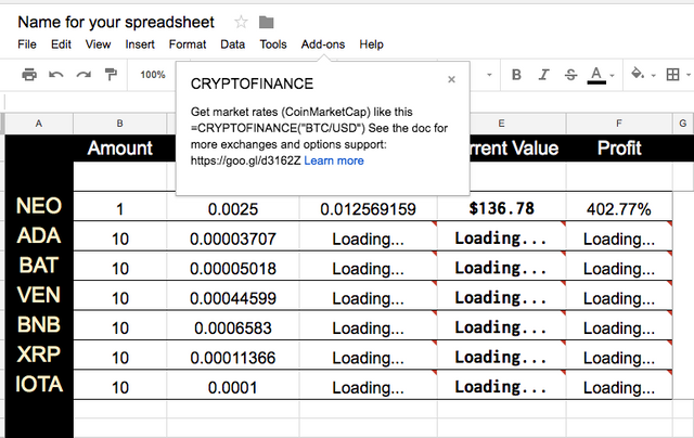
If your worksheet does not exit this load then you should do a REFRESH (Ctrl+R) on the page.

For today it is this, I hope that my example serves for someone, as well as these explanations. :D

Image from: http://yandere-simulator-fanon.wikia.com/wiki

ps: all other images are my printscreen.

You can see this post like a card in: https://channels.cc/c/d3a8ef98-3895-4372-9e23-f5ae70fabc5f