How to use SUMIF and SUMIFS in Excel
The SUM function in Excel is probably the most widely used function available. In fact it is the only formula that has its own keyboard shortcut (Alt & =). Therefore it should come as no surprise that this basic mathematical function has more powerful cousins available in Excel. These functions are know as SUMIF and SUMIFS.
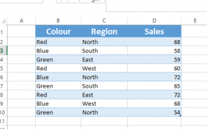
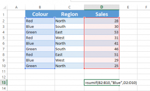
Lets say you wanted to sum a column in your spreadsheet by a specific criteria. Taking the example in the image below, lets say you wanted to sum the sales for just blue items. Using the formula =SUM(D2:D14) will result in a total for all sales. So we would need to use the function SUMIF.

SUMIF will allow you sum one column based on criteria selected in another column. In our example we can see that we want to sum column D and our criteria is in column B. The syntax for SUMIF is (=Range, Criteria, Criteria Range). Where range is the range in which you want to sum, in this case column D. The criteria is "Blue" (note how this is in "" as it is text. If you are using a cell reference there is no need to use ""). The criteria range is the range in which you will find the criteria, in this case column

But what if you wanted to sum based on two or more criteria. Our data set also contains Region, we could try and get the total sales for Blue in the North. SUMIF will only allow you sum based on one criteria. SUMIFS will allow you sum using multiple criteria.
The syntax for SUMIFS is (=Sum Range, Criteria Range 1, Criteria 1, [Criteria range 2, Criteria 2)....). As you can see this function requires the range in which you want to sum as the first range, after this you then select the cells that contain the criteria and then you specify what the criteria is. After this you can add the second and subsequent criteria.
In this video we will look at an example of SUMIFS in action. Its one thing talking about a function in Excel, but if you really want to learn and understand it, have a look at the video and then set your self out with a simple example.
Just before we get to the video, here is another excel tip. Lets say you wanted to set your self up with some random sample data. The quickest way is to select the cells in which you want to include the data and then enter the formula =RANDBETWEEN(bottom, top). For bottom and top enter the lowest and high-test number you want in your sample data. Then press CTRL & Enter to populate all of the cells.
Updated* Now includes XLOOKUP

Explore The Ultimate Excel Formulas Course

Preview Access All Areas