How to make a Sensitivity Analysis with an Excel Macro (Part 1)
I didn't get much of attention on my first post, so here it is again:
Suppose you have a business case model in a worksheet with 3 or more variables/assumptions you will like to change and see how that affects the financial results of your project. In this case I will use 9 different assumptions that will change.
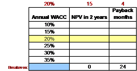
First of all you should create an extra worksheet named, say, Sensitivity. There you will make a table where you will list one by one each assumption with 3 important variables next to them: original value, row and column of the assumption you will like to change at the business case worksheet. Then, you will fill in the first column with all the other values you wish to test for this assumption, for example:

See the last row with the word "Breakeven"?. Well, that's where the macro will find the exact value of the assumption where the financial breakeven is obtained. In this case, we will use 24 months with NPV=0 to achieve this breakeven.
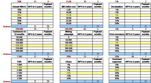
Now, replicate this table 9 times with the other assumptions in a simetrical pattern, like this:

Do you see how the corresponding original value of each assumption is highlighted in yellow? Well, that's not very important but I like my worksheets to look comprehensible... That was achieved with the "Conditional format" (when the value of the row matches the original value in top of each table).
Ok, now comes the fun part. How to fill up this table?
That will be answered in the following post if I get enough likes in this one.
Best regards!!